Gauge Magic 1 – Fuel, Temperature &
Pressure Gauge Matching / Calibration / Linearisation
Download
Link: Downloads/GaugeMagic1.zip
Purchase
Link: https://www.ebay.co.uk/itm/256132836474
(Built) https://www.ebay.co.uk/itm/256132836654
(Kit)
A simple,
effective, flexible and cheap solution to making any moving coil gauge work
accurately and linearly with any sender.
There was a recent discussion on BlatChat (the Caterham and Lotus
Seven Club Form, for those who are reading this directly on my website) on how
to correctly calibrate a fuel gauge to match a fuel tank sender. In that case
it was for an electronic dash that had calibration functions built in, but it
struck a chord with me because my own fuel gauge has always been very
non-linear, dropping very slowly over the top half of the scale and then
plummeting like a stone. I wanted to develop something for those of us who
don’t have the luxury of electronics dashes. I know there are other tools
around like the Spiyda Gauge Wizard, but they are relatively expensive and I
felt like having a go at doing something myself that was:
· Better.
· Cheaper.
· Possible to DIY.
I’ve now designed and built a few of these devices, one is installed on the fuel gauge in my car and is working really well. So I’m sharing the design details and plans here, in case anyone else wants to build one. I’m also going to be selling them in kit form very cheaply (if you fancy a bit of fun with a soldering iron) and as fully built and tested units (if you don’t) here: https://www.ebay.co.uk/itm/256132836474 (Built) https://www.ebay.co.uk/itm/256132836654 (Kit). As always, the firmware for the device and the software to configure it can be downloaded from the links on this page for free.
Design
Objectives & Features
The design I’ve come up with meets all of objectives I set myself at the start, so these now form a feature list for the device:
Basic Features
- Works with fuel, temperature and pressure gauges with no changes.
- Should work across a wide range of 12V vehicles with no changes.
- Works with a wide range of moving-coil meters (including Caterham original gauges and aftermarket gauges).
- Works with a wide range of resistive senders (including Caterham original senders and aftermarket senders).
- Allows mismatched senders and gauges to be calibrated and used together.
- Allows the gauge reading to be calibrated, corrected and linearized right across the scale.
- Works with gauges which read both forwards and backwards.
- Plug and play connectors, just plugs between back of the gauge and the loom. No wires to cut or new connections to make.
- Small and light enough to just cable-tie to the wiring (approximately 55mm x 23mm x 15mm).
- Once configured, calibration will be saved permanently in internal non-volatile EEPROM.
More
Details & Advance Features
- Simple two-step calibration.
- Calibrate the sender to read in “real units” (litres / gallons / °C or anything else you care to choose).
- Calibrate the gauge to display in the same “real units”.
- Anywhere from 2 to 20 sender calibration points.
- Anywhere from 2 to 20 gauge calibration points.
- Free Windows configuration and calibration application on my website.
- Includes a display of the current sender reading and resistance, allows you to e.g. fill the fuel tank one litre at a time, recording the resulting readings.
- Includes a slider to set the current gauge drive, allows you to work out the gauge drive numbers to put the gauge needle in any position on the scale.
- Configurable damping.
- Probably not needed with standard Caterham gauges as they are heavily damped anyway. But can add additional damping to less-damped aftermarket gauges.
- Allows the signal used for the LED and buzzer alerts to be damped separately (see below).
Alerts
- Completely configurable alert zones, each of which:
- Triggers between defined minimum and maximum “real units” values, e.g.
- One alert when fuel drops below 10 litres.
- Another alert when fuel drops below 5 litres.
- Another alert when fuel drops into the reserve zone.
- Built-in, loud piezoelectric buzzer. Configurable to:
- Turn Off.
- Sound continuously.
- Beep 1, 3, 5, 7 or 9 times.
- Beep on every alert, or just one time for each alert zone in any one journey.
- Optional outputs to drive 2 LEDs, or one bi-colour LED. Independently configurable to:
- Turn Off.
- Turn On.
- Flash.
- Drive up to two separate optional LEDs or a single bi-colour LED, e.g. red/green LED can display red/green/yellow/off.
- Configurable hysteresis to stop repeated alerts near the threshold. e.g. Will not trigger a new alert zone until you go beyond the limits of the current zone by at least 2 litres.
- Alert priorities. Control which alerts take precedence.
Construction
- Built on standard stripboard with easily available standard parts, no custom PCB needed.
- Plans for free on my website (below in this article) so you can build your own (not difficult).
- Pre-build and tested units and kits of parts for sale here: https://www.ebay.co.uk/itm/256132836474 (Built) https://www.ebay.co.uk/itm/256132836654 (Kit).
- Device firmware free to download from my website here: Downloads/GaugeMagic1.zip (file GaugeMagic1\GaugeMagic1.ino is included in the ZIP file downloaded). Source code available, so anyone who wants to can tweak it.
- Very simple to configure and calibrate over a standard USB cable.
Design & Construction
This
section covers the design and plans for building the unit. If you’re not
interested in building one and just want to use a pre-built unit you can skip
over this section and go straight to the “Installing The
Device” and “Configuring the Device” sections below.
The design is built around an Arduino Nano microcontroller. This reads the sender using a resistive divider and then drives the gauge with a PWM (Pulse Width Modulated) signal. Rather than turning the gauge only partly on as a resistive sender would do, it turns the gauge fully on but for only part of the time. This seems to work well with most analog moving-coil type gauges. The Caterham gauges are very heavily mechanically damped internally and you can drive them with relatively low frequencies, which give the best (highest resolution and most linear) gauge response. Some cheap aftermarket gauges have very little damping at all and the needle vibrates and oscillates at low frequencies. The device lets you select the drive frequency, so you can select the lowest frequency that works well with your gauge.
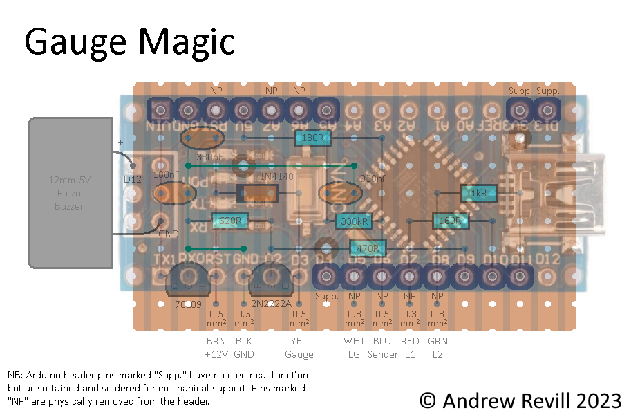
Here is the circuit diagram for the device:
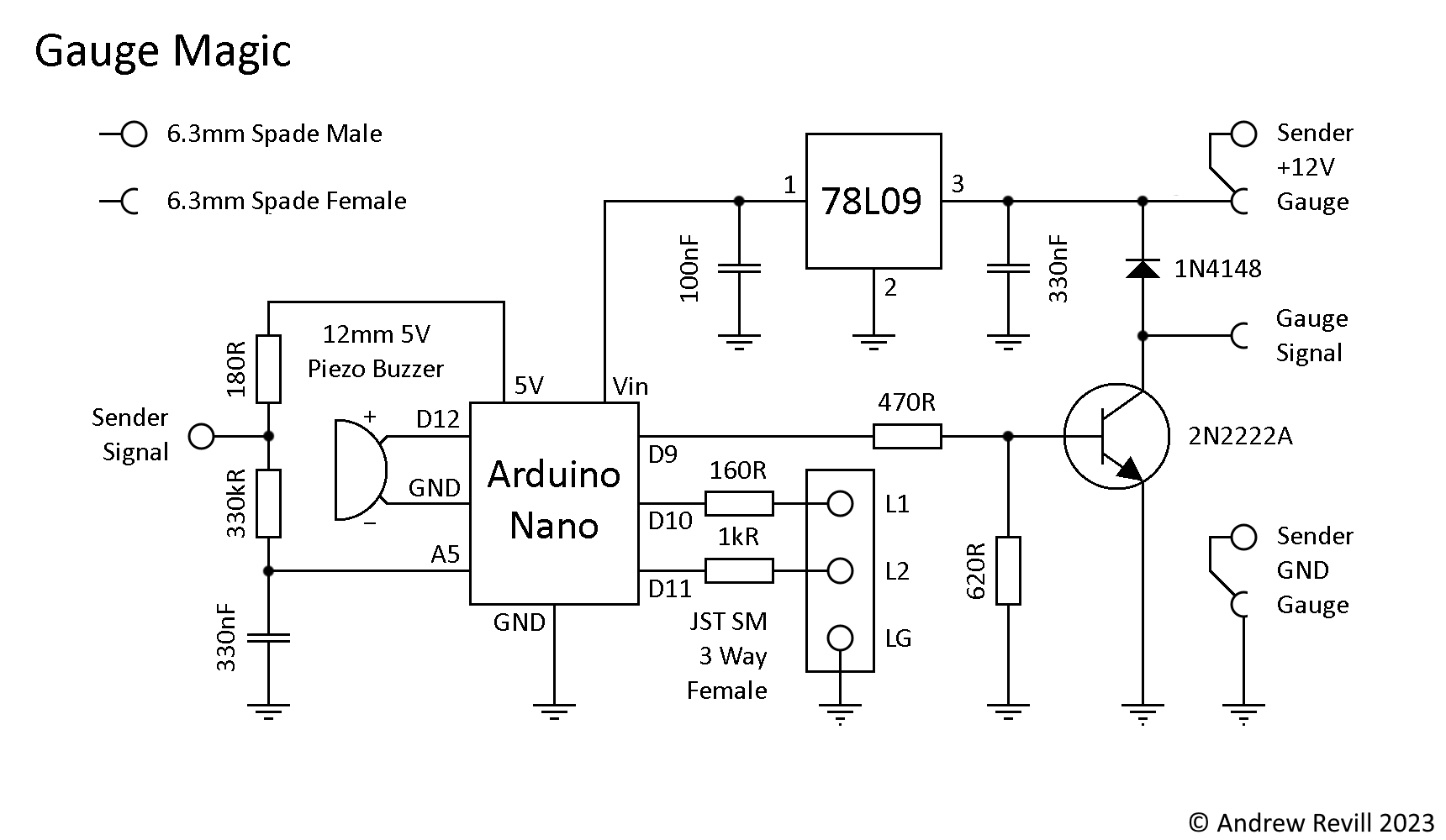
All resistors are 1/8 Watt, 1% tolerance (although the tolerance only really matters for the 180 Ohm resistor). NB: Larger 1/4 Watt resistors may not fit the circuit board design.
All capacitors are ceramic, 2.54mm lead pitch, 50V rated (or at least safely higher than battery voltage).
Running through the circuit diagram (roughly from left to right), the sender is fed with a regulated 5V supply from the internal regulator on the Arduino. This is also the reference for an analog to digital converter in the Arduino. The sender is fed through a 180 Ohm, 1% resistor, so the analog to digital converter reads the sender resistance R as a fraction of (R+180) on a scale of 0 to 1023. Any inaccuracies in the 5V supply cancel out as the same supply feeds the sender and the analog to digital converter reference voltage. A resistor value of 180 Ohms gives a good resolution over the range of resistance values commonly used for gauge senders. The table below shows the change in ADC count for a 1% change in resistance at a wide range of resistance values. You can see that the relative resolution peaks around the value of the 180 Ohm resistor chosen. If you want the device to read resistances over a very different range for some reason, just choose the value of this resistor to match.
|
Resistance |
ADC Count |
||
|
Ohms |
/ 1% Change |
||
|
20 |
0.9 |
||
|
50 |
1.7 |
||
|
100 |
2.3 |
||
|
200 |
2.5 |
||
|
500 |
2.0 |
||
|
1000 |
1.3 |
||
|
2000 |
0.8 |
||
The analog to digital converter input is fed through a 330 kilohm resistor with a 330 nanofarad capacitor to ground. These place very little loading on the sender circuit and form a low-pass filter with a time constant of about 0.1 seconds to filter out any line noise and ensure clean samples ahead of the software filtering and damping performed by the microcontroller.
The Arduino drives a piezoelectric buzzer directly and the two optional LED outputs. Because of the different semiconductors used to make them, the forward voltages and current to brightness profiles for different coloured LEDs are different. The red LED 1 wire is designed to drive a red LED with a forward voltage of around 2.1V. It is fed with 5V through a 160 Ohm resistor giving an LED current of about (5 – 2.1) / 160 = 18mA. The green LED 2 wire is designed to drive an emerald green LED with a forward voltage of around 2.5V. It is fed with 5V through a 1kR Ohm resistor giving an LED current of about (5 – 2.5) / 1000 = 2.5mA. They are primarily designed to drive a typical bi-colour, common cathode red-emerald green LED, which is really just two LEDs in one package with the negative terminals or cathodes joined together. This can then be made to show red (LED 1 On, LED 2 Off), yellow (LED 1 On, LED 2 On) or green (LED 1 Off, LED 2 On). In these LEDs the emerald green LED tends to be a lot brighter at the same current and requires a much lower current to achieve a good optical balance with the red LED and to produce anything that looks like a shade of yellow when both LEDs are lit together. The red wire will drive a green LED very brightly and the green wire not light a typical red LED very brightly at all. The forward voltage and brightness of a blue LED are close enough to those of a green LED to be able to satisfactorily drive a blue LED off the green LED 2 wire e.g. for use as an under-temperature warning. I can supply suitable bi-colour LEDs on JST SM male leads here: https://www.ebay.co.uk/itm/256132884131. Adjust the values of the resistors if you want the LEDs brighter or dimmer (but do not exceed the absolute limits of 40mA per Arduino pin, 200mA total for the Arduino but only 100mA total for the 78L09 regulator). Because the resistors are included on the board, you can use standard LEDs rather than 12V types with built-in series resistors.
The Arduino also drives a 2N2222A NPN open-collector transistor switch with the PWM signal, which drives the gauge. As the gauge coil is inductive, a 1N4148 diode clamps any switching transients. The gauge current ramps up when drive is first applied, and ramps down when drive is removed as the stored energy is dissipated in the diode. Because of the significance of the “end effects” when the drive turns on and off, different frequencies will drive the gauge to different positions even with the same duty cycle, an effect which is more noticeable at higher frequencies where the end ramps tend to dominate over the steady-state on and off portions of the waveform.
A 78L09 linear regulator and associated capacitors step the 12-14.5V supply voltage from the vehicle down to 9V for the Arduino. At worst case the Arduino will draw 19mA, the two LEDs 21mA and the buzzer 14mA giving a total current draw of 54mA which is well within the current limit of 100mA for the 78L09, and at a supply voltage of 14.5V this gives a peak power dissipation in the regulator of 248mW which also falls well within the specified limit of 500mW. The Arduino is rated for 40mA per pin and 200mA total current sourced.
Parts List
Below is a complete list of the parts necessary to build the device. All of these parts are cheap and readily available. I can supply them as a complete kit here: https://www.ebay.co.uk/itm/256132836654.
|
Arduino Nano Clone & Headers (Unsoldered) |
|
Stripboard 15 Strips by 8 Holes |
|
78L09 Voltage Regulator IC |
|
2N2222A NPN Transistor |
|
1N4148 Diode |
|
Active (DC) Piezo Buzzer |
|
160R Resistor |
|
180R Resistor |
|
470R Resistor |
|
620R Resistor |
|
1kR Resistor |
|
330kR Resistor |
|
100nF Capacitor |
|
330nF Capacitor X 2 |
|
20mm Non-Adhesive 2:1 Heat-Shrink Tubing X 55mm |
|
Male Spade Terminals X 3 |
|
3mm Non-Adhesive 2:1 Heat-Shrink Tubing X 3 X
15mm |
|
Female Spade Terminals & Sleeves X 3 |
|
Tinned Copper Wire 0.45mm |
|
Pre-Wired 3-Way JST SM Female Connector on 0.3mm²
Cable |
|
0.5mm² Cable, Brown X 20cm |
|
0.5mm² Cable, Black X 20cm |
|
0.5mm² Cable, Yellow X 20cm |
|
0.5mm² Cable, Blue X 17cm |
Construction
The components are assembled on a small piece of stripboard, with 15 strips by 8 holes:
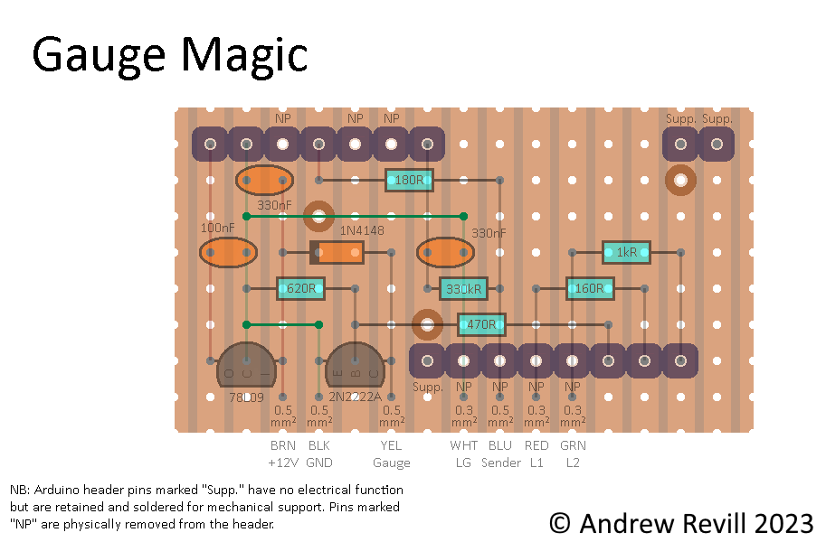
A few points to note:
· The brown circles indicate track spot cuts, where the copper tracks are cut at particular holes. This can be done with a stripboard spot-cutter tool or a 3.5mm drill bit (by hand). There are only 3 cuts required.
· The green wires are tinned copper wire jumpers.
· Note the correct orientation of the 1N4148 diode (black cathode stripe to the left) and the 78L09 regulator and the 2N2222A transistor (flat package side downwards).
· The 78L09 and 2N2222A must sit as low as possible on the board in order to allow the Arduino to be soldered onto the headers above them. Push them firmly down into place before soldering.
· The headers supplied with Arduino are cut down to lengths of 2, 7 and 8 pins as shown above.
· 3 pins are removed from 7-pin header and 4 pins are removed from the 8-pin header as shown. The pins are removed completely from the plastic housing. These can gently worked out by gripping them with a pair of wire cutters.
· The headers are soldered flush to the board with the long ends of the pins upwards for mounting the Arduino and short ends through the board and soldered.
· Some of the Arduino pins are electrically unused but remain in the headers and are soldered as normal to provide mechanical support.
· The spots in the bottom row indicate where wires are attached. Wires are soldered directly to the board and routed out to the right in the bottom right-hand corner. The heat-shrink tubing used to encapsulate the device provides adequate mechanical support.
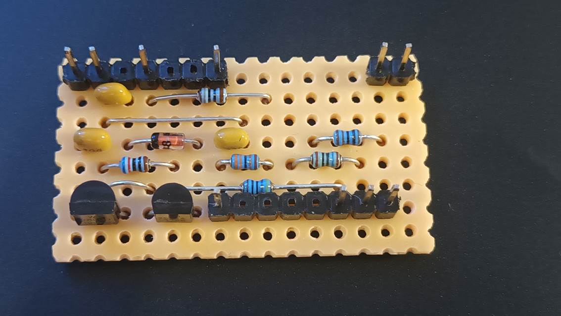
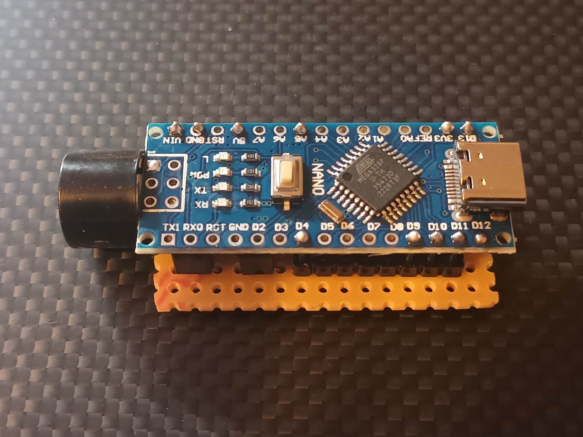
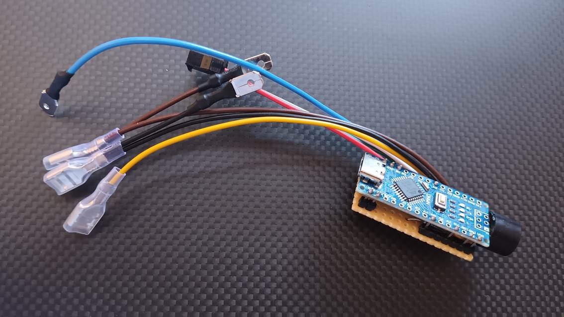
Here is a photograph of a completed circuit board for reference:
The piezo buzzer unit is then soldered to the UNDERSIDE of the Arduin nano as show below. Note that the piezo buzzer MUST be of the ACTIVE type (contains its own internal oscillator chip and only requires a DC power supply, not an audio frequency square wave or similar drive signal from the Arduino) and must be specified for use with a 5V supply.
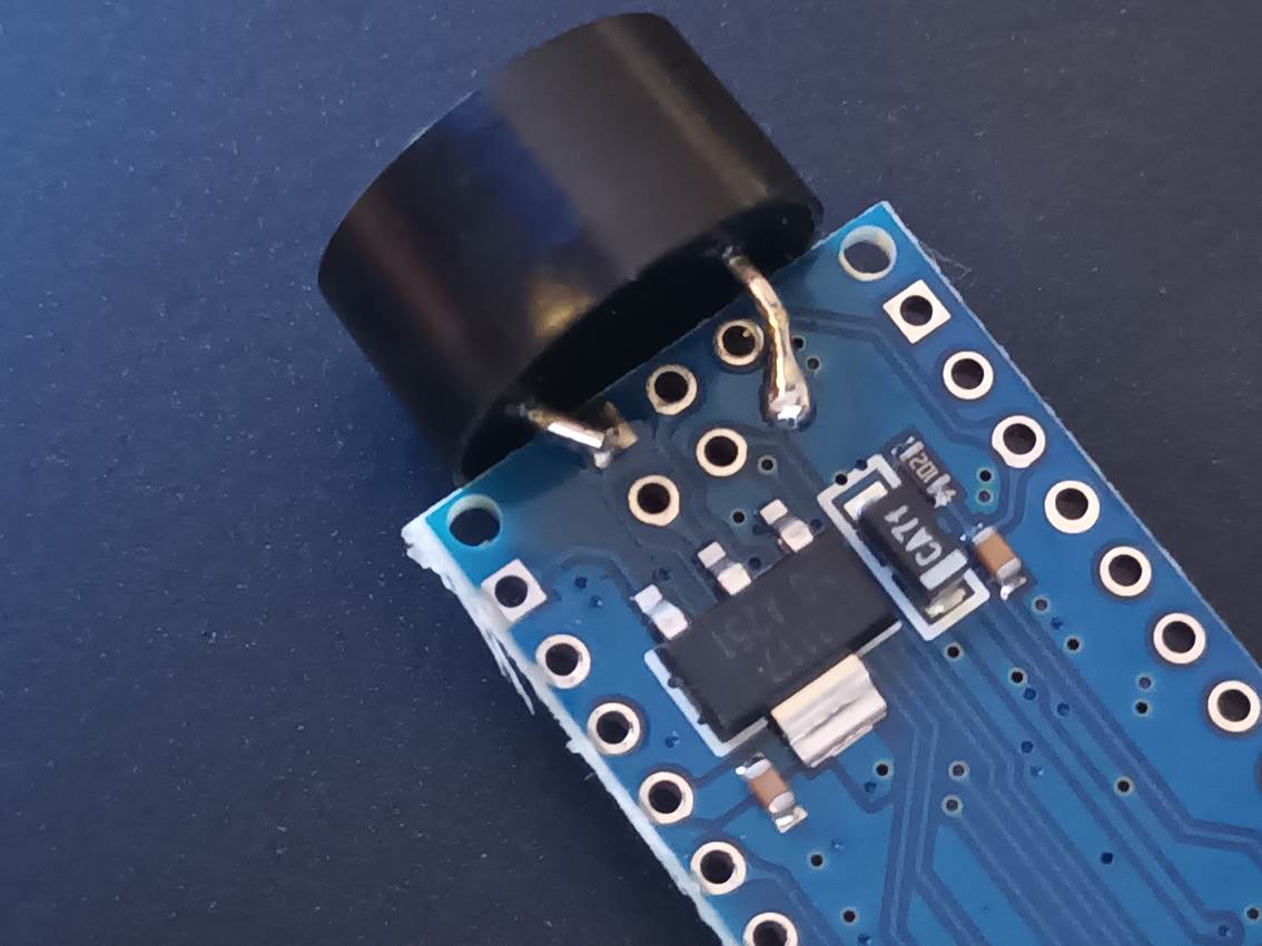
The leads need to be bent to shape. Note that the polarity is important, and the positive lead which is usually LONGER as supplied is cut very short and soldered to the pin hole shown in the outer row whereas the negative lead which is usually SHORTER as supplied is simply bent round to reach the pin hole shown in the inner row, clearing the hole in the outer row.
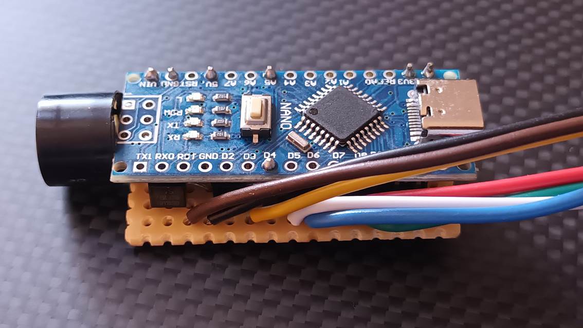
Once the two boards have been completed and checked carefully against the designs (as once soldered together it is very difficult to remove the Arduino to make corrections without damaging anything), the Arduino is then soldered onto the headers, with the piezo buzzer downwards, as shown below. If the 78L09 and 2N2222A have been mounted low down to the board as described, it will be possible to seat the Arduino square on the header pins with enough pin protruding to solder from the top:
Here is a photograph of the two soldered together:
The device is then wired as shown below:
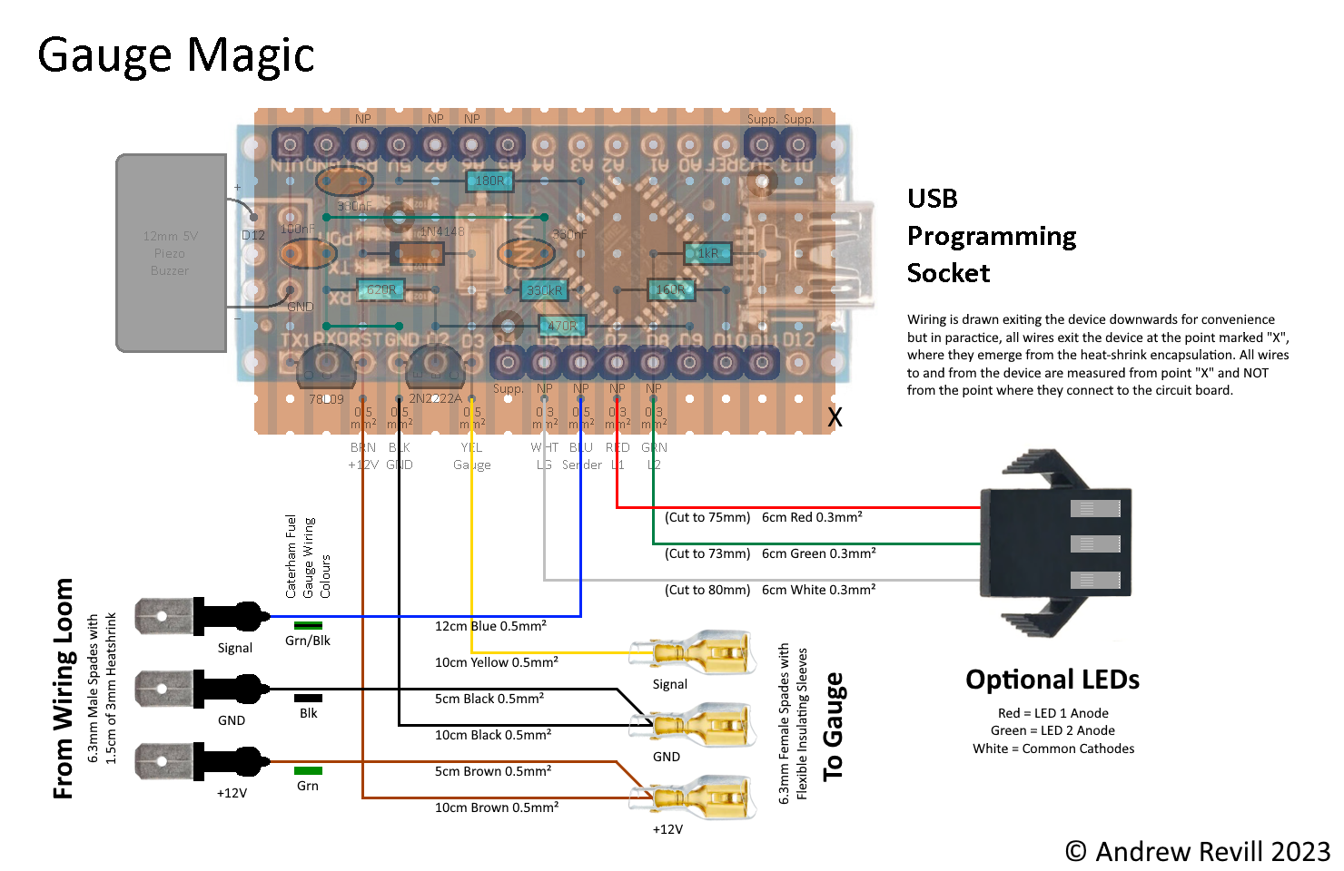
The LED socket comes pre-wired with 0.3mm² cable in the colours shown. These need to be carefully cut to length so that the wiring will lie flat and will not be under strain when soldered. Suggested wire lengths are all measured from the point marked “X” through which the cables are routed as they leave the device. In order to achieve a 6cm wire length for the LED socket, the red wire needs to be cut to length 75mm, the green wire to length 73mm and the white wire to length 80mm. The remaining wires to the loom and gauge use 0.5mm² for robustness. It may be easiest to solder the 0.5mm² wires to the board first, then the LED wires, as the LED wires cannot be bent aside so easily. Be careful not to bend the wires backwards and forwards sharply to avoid fracturing them where they are soldered to the board; the solder will wick into the wire and make it relatively brittle. Once the device is complete, the heat-shrink encapsulation holds the wires firmly in place, provides the necessary mechanical support and prevents movement at the soldered joints.
Once the wires have been soldered to the board, the outer insulating encapsulation may be applied. This is done with a 55mm length of non-adhesive, 20mm diameter, 2:1 ratio heat-shrink tubing. This will initially appear to be too long, but if you align end of it with the edge of the USB programming socket and then apply heat working forwards towards the buzzer it will shrink into place correctly, providing insulation, protection and mechanical support. Ensure that the USB socket remain accessible. The use of non-adhesive heat-shrink tubing allows it to be cut away and replaced easily if any repairs are required.
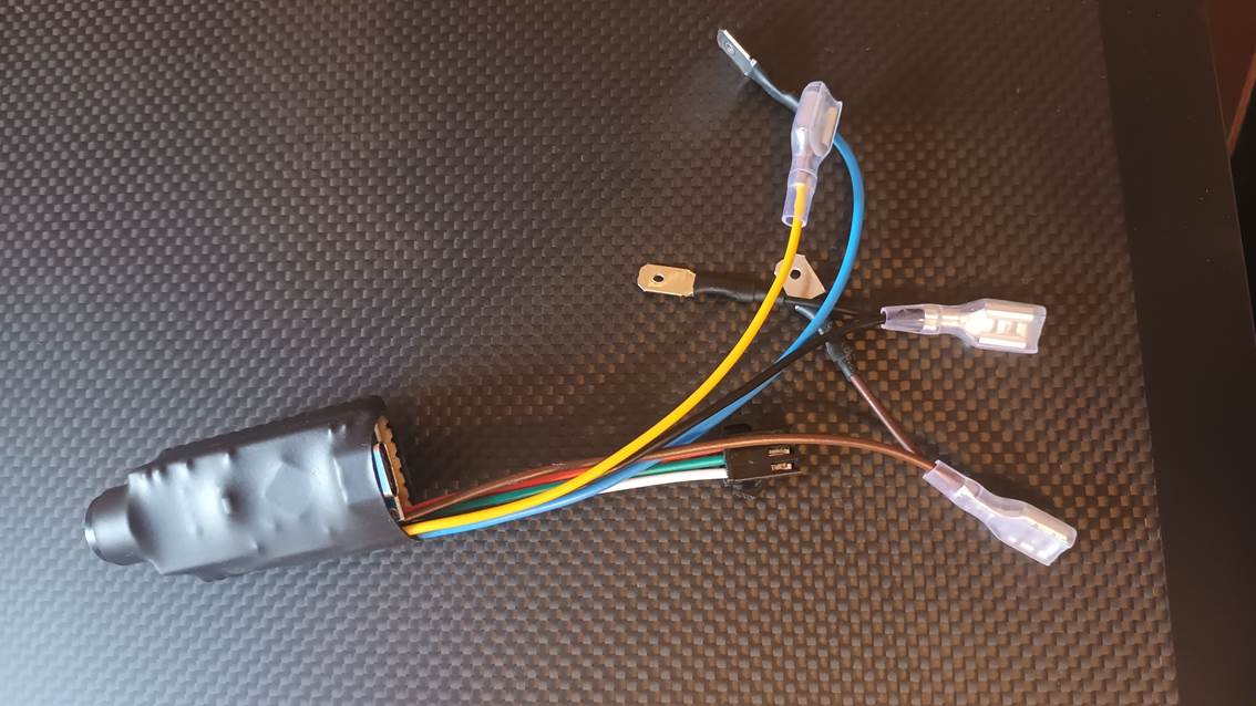
For a Caterham fuel or temperature gauge, and for many other common gauges, the three connections to the back of the gauge are made with 6.3mm female spade terminals with flexible insulating rubber boots. The supply and ground terminals are crimped with two wires each, such that a short 5cm length of wire runs back to the corresponding loom connector. The three connections to the wiring loom are made with 6.3mm male spade terminals with 1.5cm of 3mm 2:1 non-adhesive heat-shrink insulation covering the non-mating parts. These simply push into the original connector for the gauge. In the case of a Caterham, the loom wiring colours are shown above for identification. When wired as above, the whole device may simply be inserted between the wiring loom connector and the back of the gauge without any need to cut any connections, modify any wiring or add any new connections (other than the optional LED wiring, if required).
Installing The Device
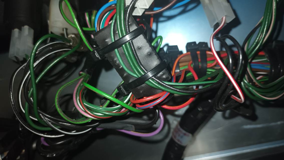
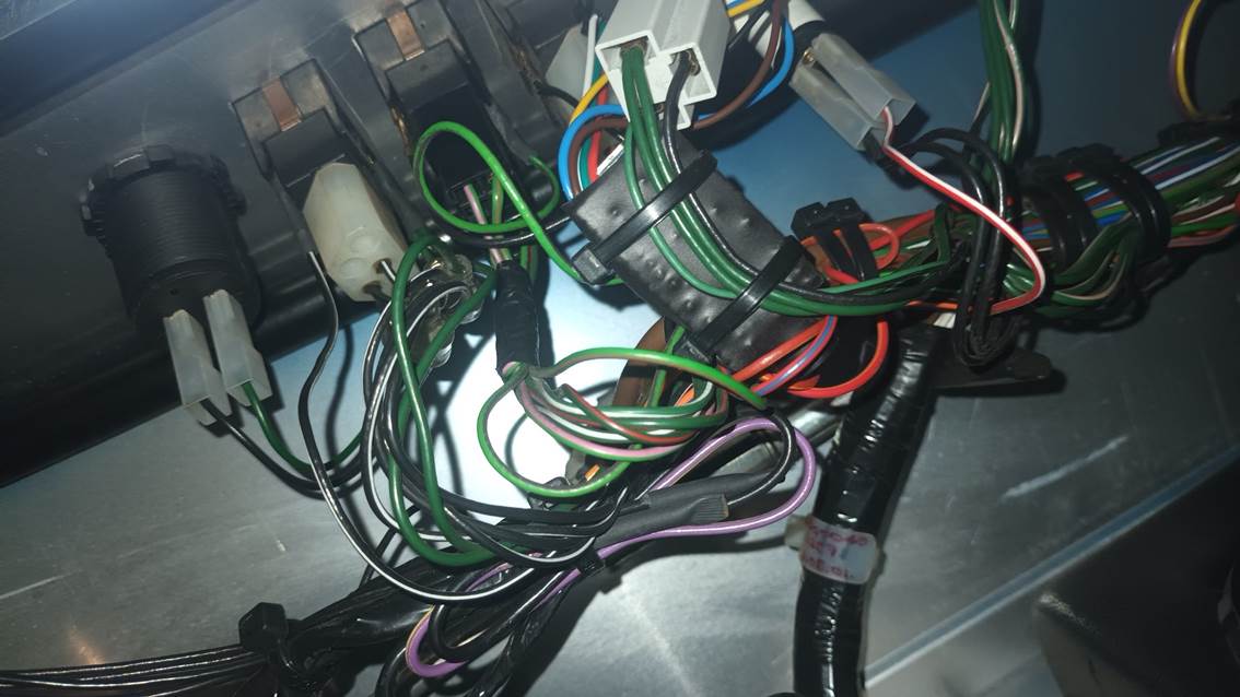
Installing the device is very simply. Assuming a Caterham gauge or a gauge with similar connectors, simply pull the connector off the back of the gauge, push the three male spade terminals into the connector (ensuring that you get them in the correct positions), push the three female spade terminals onto the back of the gauge, and then cable-tie the device into the existing loom wiring out of the way behind the dash. The brown wires are the +12V supply, which in the Caterham wiring loom are coloured green. The black wires are the ground connection, which in the Caterham wiring loom are also coloured black. The blue wire connects to the sender, which in the case of a Caterham fuel gauge is coloured green/black in the loom. The yellow wire goes to the sender position on the gauge itself. WARNING: In the middle of the Arduino Nano board is a reset push-button. The heat-shrink tubing will not apply enough pressure to activate this. Be careful not to cable-tie the device tightly with this pressed hard against the existing wiring or it may permanently hold the device in reset. Try to ensure that the USB socket remains accessible to allow reconfiguration of the device in situ.
Configuring The Device
Before diving into the detailed example of exactly how I used this to calibrate my fuel gauge, here is a simple summary of the steps involved in calibrating the device:
· Download the configuration utility.
· Connect to the device over USB cable by selecting the correct COM port.
· Use the Sender Calibration tab to enter the calibration of the sender in terms of “real units”. In this tab, the current sender reading is displayed to help you.
· Use the Gauge Calibration tab to enter the calibration of the gauge in terms of “real units”. In this tab, the utility drives the gauge with the numbers you enter.
· Use the Response Damping tab to set the response times for the gauge and for alerts.
· Use the LED / Buzzer Alerts tab to configure any alert zones you want.
If you want, you can just dive straight in and play around with configuring the device. If you want a more detailed explanation, I’ve gone through the details of how I calibrated my fuel gauge below. You can use this as an example. The process is basically the same for calibrating a temperature or pressure gauge.
If you have built the device yourself, you will need to upload the Gauge Magic firmware to the device. Ready-built devices and parts kits will come with this already installed. To install the firmware, you will need to download the Arduino IDE from https://www.arduino.cc/en/software, and download the firmware sketch file here: Downloads/GaugeMagic1.zip (file GaugeMagic1\GaugeMagic1.ino is included in the ZIP file downloaded). Use the IDE to open the firmware sketch file and upload it to the device in the normal way.
Detailed Example
In order to configure and calibrate the device, download the configuration utility here: Downloads/GaugeMagic1.zip (files GaugeMagic1.32.exe (32-Bit) and GaugeMagic1.64.exe (64-Bit) are included in the ZIP file downloaded). 32-bit and 64-bit versions of the application are provided, use whichever is appropriate to the version of Windows you are running. You will need a USB cable (usually Type C). Connect the device to a Windows PC using the USB cable. It will connect as a virtual COM port.
When you launch the configuration utility you should see something like this:
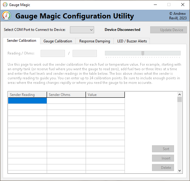
Everything is greyed out and disabled because it is not connected to a device. The device should appear as a new COM port in Windows when the USB cable is connected. To connect to the device, simply select the COM port from the dropdown list. If you see multiple COM ports and you’re not sure which one is the device, just unplug the USB cable from the device and see which one disappears. The COM port for the device will only show in the list when it is connected. Once you select the device COM port, you should see something like this:
The device ships with a default calibration, which is the one I used on my car and which is shown in the examples in this article. This probably won’t be right for your car, but it at least means that the device will be functional and you can experiment with it.
There are 4 main tabs along the top:
· Sender Calibration – This is where you enter the calibration of sender reading / resistance to “real units”.
· Gauge Calibration – This is where you enter the calibration of “real units” to gauge drive.
· Response Damping – This is where you can configure the damping or smoothing for the gauge and alert responses.
· LED / Buzzer Alters – This is where you configure the alert zones and how you want the buzzer and LEDs to behave.
· (Device Log) – This only shows up if you pass “/L” as a parameter when running the application. It shows a log of the communications with the device and was really designed for me to use during development.
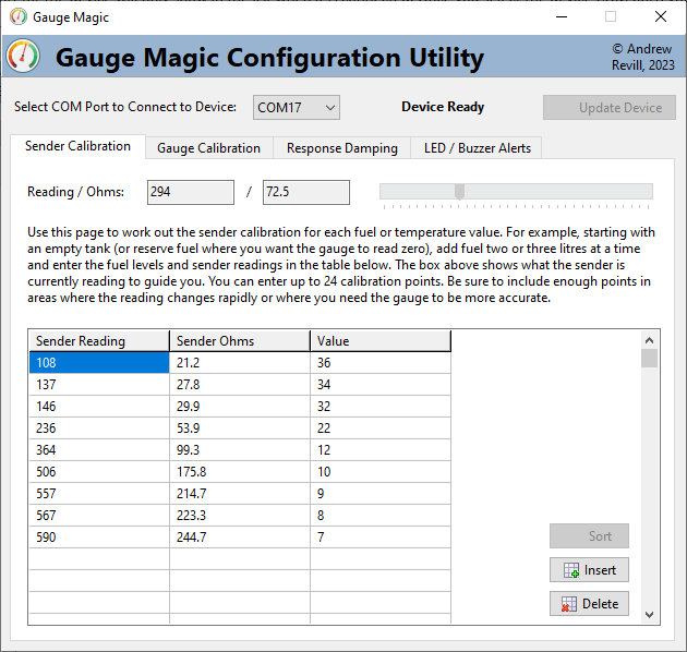
At the top of the Sender Calibration tab, you can see the current sender reading (analog to digital converter output in the range 0-1023) and calculated sender resistance in Ohms. You can use this to work out the sender calibration and how the sender responds to different fuel / temperature / pressure values.
Below that is a table where you can enter the sender values and corresponding “real units” values. NB: It really doesn’t matter what units you want to use here, you can use anything sensible. For a fuel gauge it makes sense to use something like litres, but cubic centimetres, pints, gallons or miles range would all work fine. You don’t even need to tell it what the units are, just be sure to use the same units in the Sender Calibration and Gauge Calibration tabs and everything will work out fine.
A note about sender readings and sender resistances: The device works directly off the sender readings, which are numbers in the range 0 to 1023. If you are doing this process from scratch, it is more accurate and more consistent to forget about sender resistances in Ohms and work directly in terms of sender readings. However, some people may already have checked their fuel sender calibrations and may already have a useable set of numbers in terms of sender resistance in Ohms. In this case, you can key sender resistances in Ohms into the second column of the table; these values are then converted to the nearest sender reading and this is what the device will use.
Here’s how I went about calibrating the fuel tank sender in my 2001 Caterham 7 SV:
I started by draining the tank to completely empty, or at least to a reference point that was lower than I would ever want to go on the road. I did this by disconnecting the fuel return hose from the fuel rail and running a couple of metres of fuel hose from the fuel rail to a large 20 litre Jerry can, then starting from less than half a tank I ran the engine until the fuel pressure in the fuel rail started to fluctuate and the engine started to stumble. At this point my tank was pretty much right down to the bottom and all of my petrol was pumped out into the Jerry can. I would never want to run anything like this low on the road as the fuel pump was picking up air even sitting still and level, so that was as low as I needed to go. I then reconnected the fuel return hose and started adding fuel one litre at a time, noting the sender reading after each litre was added. I gave the car a bit of shake after adding each litre just to ensure that the fuel tank sender float had settled and wasn’t sticking.
|
Litres |
|
|
From |
Sender |
|
Cutout |
Reading |
|
0.0 |
|
|
1.0 |
|
|
2.0 |
|
|
3.0 |
|
|
4.0 |
|
|
5.0 |
|
|
6.0 |
590 |
|
7.0 |
590 |
|
8.0 |
567 |
|
9.0 |
557 |
|
10.0 |
506 |
|
11.0 |
434 |
|
12.0 |
364 |
|
13.0 |
346 |
|
14.0 |
334 |
|
15.0 |
324 |
|
16.0 |
305 |
|
17.0 |
294 |
|
18.0 |
284 |
|
19.0 |
265 |
|
20.0 |
256 |
|
21.0 |
245 |
|
22.0 |
236 |
|
23.0 |
226 |
|
24.0 |
217 |
|
25.0 |
207 |
|
26.0 |
198 |
|
27.0 |
189 |
|
28.0 |
180 |
|
29.0 |
171 |
|
30.0 |
163 |
|
31.0 |
154 |
|
32.0 |
146 |
|
33.0 |
138 |
|
34.0 |
137 |
|
35.0 |
123 |
|
36.0 |
108 |
|
37.0 |
108 |
|
38.0 |
|
|
39.0 |
|
|
40.0 |
|
|
40.5 |
Below 7 litres the sender reading remained at 590, and the sender was clearly at the bottom of its useable travel. Above 36 litres, the sender reading remained at 108, the sender was clearly at the top of its useable travel and the last few litres to brim full were unreadable. These were the working limits of the sender and there was nothing I could to read the fuel level accurately outside of them.
I then plotted these as a chart in Excel:
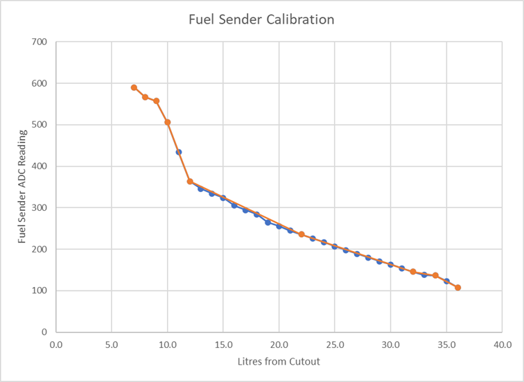
You can see how very non-linear the response is below about 12 litres due to the irregular shape of the fuel tank. But it’s also easy to see that the response is close to being a small number of straight-line segments, and using just 9 calibration points instead of one per litre (the orange points and line above), I could get very close to the measured sender calibration curve (the blue points and line). The device allows you to specify up to 20 calibration points (and you need a minimum of 2), but in reality, you won’t need anything like that. To be honest I could have used a lot fewer than 9 points and still been as accurate as I would ever need.
So I simplified the above calibration curve to the following 9 points and keyed it into the table in the configuration utility. Note that the device expects the calibration points to be in ascending order of sender reading and the points I had were in ascending order of fuel level and descending order of sender reading, but this doesn’t matter as the configuration utility will sort the points itself when you write them to the device.
|
Sender |
Litres |
|
Reading |
Nominal |
|
108 |
36 |
|
137 |
34 |
|
146 |
32 |
|
236 |
22 |
|
364 |
12 |
|
506 |
10 |
|
557 |
9 |
|
567 |
8 |
|
590 |
7 |
NB:
Whenever you have made changes to settings or calibrations, you need to click
Update Device to write these to the device itself. Until you do that, nothing
is saved. When you update the device, all changes you have made are written to
the device and stored in permanent memory.
I then moved on to calibrating the gauge itself.
I decided I wanted the gauge to read as follows:
|
0 to 7 Litres |
Unreadable, Unusable |
|
7 to 10 Litres |
Readable Reserve |
|
10 to 36 Litres |
Readable Tank |
|
36 to 40 Litres |
Unreadable Tank |
The SV tank supposedly has 6 litres of unusable fuel at the bottom. As I was fairly sure I’d run the tank pretty much to empty (both because the engine was quitting and because I was able to add 40.5 litres before the tank was full) and because I had found the bottom 7 litres to be unreadable on the sender, I decided to call the last litres of the tank unusable and configure the gauge so that the very bottom of the red reserve zone corresponded to 7 litres. I then decided that I would allow 3 litres for the red reserve zone, taking me to 10 litres at the “Empty” mark on the gauge, which left 30 litres to be scaled equally across the gauge scale from the “Empty” mark to the “Full” mark. This did mean that that the gauge would never quite read full as the last few litres to full were not readable on the sender, but this was a compromise I was happy to accept. Of course, all of this was my personal choice, and you are free to scale your gauge however you choose.
That gave me a target gauge calibration of:
|
Red |
7 |
|
Empty |
10 |
|
1/8 |
13.75 |
|
¼ |
17.5 |
|
3/8 |
21.25 |
|
½ |
25 |
|
5/8 |
28.75 |
|
¾ |
32.5 |
|
7/8 |
36.25 |
|
Full |
40 |
At the top of the Gauge Calibration tab there is a box to select the gauge drive frequency and the drive level. When you select this tab, the fuel gauge will stop displaying the actual fuel level and will display the value set by the drive level entered. This allows you to manually manipulate the gauge reading to explore the calibration and drive numbers required.
First of all you need to select an appropriate drive frequency. Available frequencies range from 15Hz to 15625Hz. The rule is simple; lower frequencies give better resolutions and a more linear response, but higher frequencies give a steadier needle reading if the gauge isn’t sufficiently damped. So choose the lowest value you can which doesn’t result in any discernible vibration of the gauge needle. In my case, the Caterham gauges are very heavily damped and to be honest I’m not sure I could see any vibration even at the lowest frequency, but as I wasn’t 100% sure I went got 61Hz to be safe. Especially at higher frequencies the frequency will significantly affect the gauge response, so if you change the frequency you are using then you will need to calibrate the gauge again and the gauge calibration numbers you have already collected will no longer be correct (this ONLY affects the gauge calibration, NOT the sender calibration, which will remain fixed even if you change gauge frequencies). One other small consideration; the gauge mechanism actually works very much like a small speaker! Using frequencies in the middle of the audible range may cause the gauge to hum very quietly. This is not something you would notice in most cars with the engine running but in a quiet garage you can hear it.
Next, use the Drive edit box (or drag the slider to the right of it) to find the drive numbers needed to force the gauge to display each of the positions in your calibration. As you increase the number, or drag the slider to the right, the gauge will usually move to the right. As you decrease the number, or drag the slider to the left, the gauge will usually move to the left. So it’s quite straightforward to find the numbers you need to put the gauge at 1/4 scale, 1/2 scale or any other position. However, I found there were three complicating factors to bear in mind:
1. The gauge is quite heavily affected by the weight of the needle. If you hold the gauge at different angles, it will read differently, even with the same drive. So it’s important to do the calibration with the gauge in place in the dash, sitting at its usual angle.
2. The Caterham gauges are VERY heavily damped. This means they are very slow to settle at their final position. To get the right numbers you need to change the drive and wait at least 30 seconds to a minute to see where the gauge will finally settle.
3. There seems to be quite a bit of “stiction” in the gauges. The need stops moving just before it reaches the correct point. So the number you need to drive the gauge to 1/4 will be different depending on whether you are moving it up from 0, or down from 1/2. I decided to find one set of numbers working upwards and one set of numbers working downwards and to take the average for each point, as in real life I think vibrations of a running car will overcome the stiction and allow the gauge to settle in the correct position.
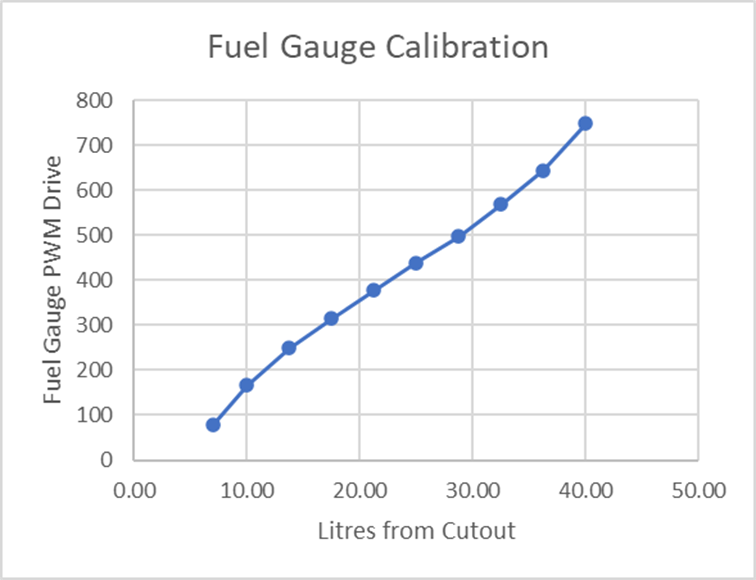
These are the numbers I ended up with. As you can see from the chart below, the gauge response is a lot more linear than the sender response:
|
Gauge |
Litres |
Rising |
Falling |
Average |
|
Red |
7 |
80 |
80 |
80 |
|
Empty |
10 |
167 |
166 |
167 |
|
1/8 |
13.75 |
255 |
242 |
249 |
|
1/4 |
17.5 |
324 |
306 |
315 |
|
3/8 |
21.25 |
390 |
365 |
378 |
|
1/2 |
25 |
450 |
427 |
439 |
|
5/8 |
28.75 |
509 |
486 |
498 |
|
3/4 |
32.5 |
579 |
558 |
569 |
|
7/8 |
36.25 |
655 |
635 |
645 |
|
Full |
40 |
752 |
745 |
749 |
`
I then entered these average numbers (litres of fuel and average drive) into the Gauge Calibration table in the configuration utility.
Reminder:
Whenever you have made changes to settings or calibrations, you need to click
Update Device to write these to the device itself. Until you do that, nothing
is saved. When you update the device, all changes you have made are written to
the device and stored in permanent memory.
At this point, your gauge should be scaled and reading correctly. But there are a few other things you can configure.
The Response Damping tab lets you set the speed (or time scale) on which the gauge and alerts respond.
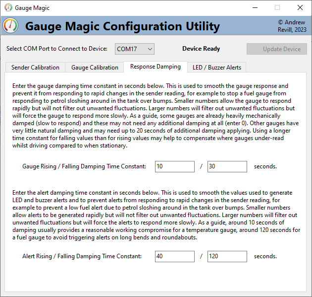
This allows you add damping to a gauge which is under-damped and so prevent the gauge from responding to the fuel sloshing around in the tank. It’s not quite the same as genuine mechanical damping in the gauge itself as it won’t prevent the gauge needle from wobbling when the gauge is shaken about, but it will prevent the gauge from responding too quickly to transient changes in the measured fuel level. Separate time constants are provided for rising and falling values. Using a longer time constant for falling values than for rising values may help to compensate where gauges under-read whilst driving compared to when stationary, as it will tend to result in the gauge reading slightly above the true average reading when the sender signal is fluctuating a lot. See Other Observations below. If you set the rising and falling time constants to the same number, then any changes in the rising number automatically update the falling number.
Separate damping is provided for the calculated average value used to drive the LED and buzzer alerts, described below. This is used to prevent for example a low fuel buzzer warning being triggered on a long bend or roundabout where the fuel is thrown to one side of the tank and the sender temporarily reads low. Fairly long damping time constants are appropriate here for a fuel gauge, where you would want the alerts to be based on the true long-term average level of the fuel in the tank and unaffected by fuel sloshing around. Much shorter time constants may be appropriate when used with a temperature gauge where these fluctuations would not occur and where you might want an over-temperature alert to occur quickly.
Finally, the LED / Buzzer Alerts tab lets you define and configure audible and visible alerts for low fuel, under- or over-temperature etc.
The device contains a small built-in piezoelectric buzzer. This is loud and piercing enough to get your attention when installed behind the dash in Caterham being driven with earplugs in! If the unit is being installed in a quieter cockpit environment, you can significantly tone down the buzzer with a piece of sticky tape over the hole in the end of it. When configured to beep N times, the buzzer beeps for approximately half a second, once per second. The device can also drive one or two external LEDs for a visual alert, as described below.
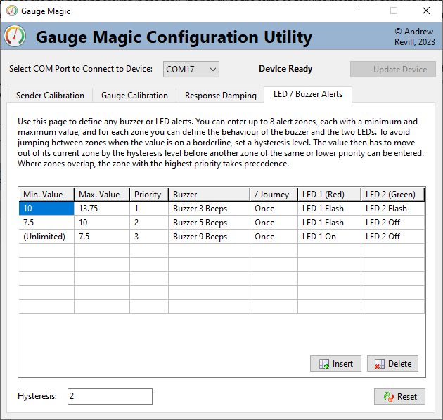
You can define up to 8 “alert zones”. Each alert zone is defined by a minimum and maximum value, in the same “real units” you chose when calibrating the sender and gauge (e.g. litres, NOT sender reading numbers). Looking at the example show above:
· When the fuel level falls to 13.75 litres (which corresponds to the 1/8 mark on my gauge) the buzzer will beep 3 times and a yellow LED will start flashing (in my car I’m using a bi-colour LED which can show red or green if one LED is turned on, or yellow if both LEDs are turned on).
· When the fuel level falls further to 10 litres (which corresponds to the Empty mark on my gauge) the buzzer will beep 5 times and the LED will turn to flashing red instead of yellow (as I turn the green LED off at this point).
· When the fuel level falls further to 7.5 litres (which corresponds roughly to what I regard as potentially unusable at the bottom of the red reserve on the gauge, plus a 0.5 litre margin) the buzzer will sound 9 times and the red LED will light solidly. I added the 0.5 litre margin to the 7-litre unusable level as I knew the sender bottomed out at this level, so with a bit of bouncing around the long-term average reading might never quite settle to the very lowest sender reading and I wanted to ensure that the final “emergency” alert sounded reliably.
In order to prevent repeated alerts when you are close to the borderline between zones, you can set a Hysteresis level. In the example above this is set to 2 litres. This means that once an alert zone has been entered, the fuel level must move at least 2 litres outside of that alert zone before the device will consider a different alert. Combined with a long damping time constant for the alert value, this will usually prevent the same alert triggering more than once. However, under extreme conditions, especially where the fuel tank sender is mounted at one side and where the fuel level reading may be heavily dependent on which direction the vehicle is turning, the device may register a low fuel alert a little early on a long bend, then return to normal after some time driving straight. Although the LED alert will then display for a short time then stop, to avoid distraction you can configure the buzzer to sound only once for each alert zone in any one journey. A “journey” ends when you turn the ignition off (assuming that the gauge is wired to receive power only with the ignition turned on as it usually should be).
Particularly in the case of fuel gauge, adding enough hysteresis to prevent repeated alerts may significantly affect the fuel levels at which the alerts are triggered. Taking the example above:
· When the fuel level falls to 13.75 litres, the first alert triggers. This applies down to 10 litres.
· When the fuel level falls to 10 litres, the second alert should trigger. But the 2 litres hysteresis requires the fuel level to fall 2 litres below the first alert zone, or 8 litres, before it will trigger the second alert.
To get around this, alert zones are given priorities, which override the hysteresis. With the priorities shown in the example above:
· When the fuel level falls to 13.75 litres, the first alert triggers.
· When the fuel level falls to 10 litres, the second alert triggers immediately because it has a higher priority (priority 2) than the current (first) alert (priority 1).
· The fuel level would then need to rise again from 10 litres to 12 litres (2 litres hysteresis) in order to cancel the second alert and return to the first alert.
Optional
LEDs
The alerts can be used to drive up to 2 external LEDs. The LED outputs are via a 3-way JST SM female connector. This has wires colour coded red, green and white. The red and green wires are the positive / anode connections for the two LEDs, the white wire is the common negative / cathode and is internally connected ground.
IMPORTANT: Because of the different semiconductors used to make them, the forward voltages and current to brightness profiles for different coloured LEDs are different. The red LED 1 wire is designed to drive a red LED with a forward voltage of around 2.1V. It is fed with 5V through a 160 Ohm resistor giving an LED current of about (5 – 2.1) / 160 = 18mA. The green LED 2 wire is designed to drive an emerald green LED with a forward voltage of around 2.5V. It is fed with 5V through a 1kR Ohm resistor giving an LED current of about (5 – 2.5) / 1000 = 2.5mA. They are primarily designed to drive a typical bi-colour, common cathode red-emerald green LED, which is really just two LEDs in one package with the negative terminals or cathodes joined together. This can then be made to show red (LED 1 On, LED 2 Off), yellow (LED 1 On, LED 2 On) or green (LED 1 Off, LED 2 On). In these LEDs the emerald green LED tends to be a lot brighter at the same current and requires a much lower current to achieve a good optical balance with the red LED and to produce anything that looks like a shade of yellow when both LEDs are lit together. The red wire will drive a green LED very brightly and the green wire not light a typical red LED very brightly at all. The forward voltage and brightness of a blue LED are close enough to those of a green LED to be able to satisfactorily drive a blue LED off the green LED 2 wire e.g. for use as an under-temperature warning. I can supply suitable bi-colour LEDs on JST SM male leads here: https://www.ebay.co.uk/itm/256132884131.
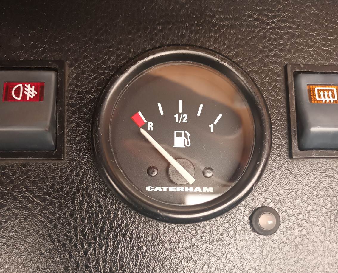
Here's a picture of the gauge and bi-colour LED in my car:
Other
Observations
One thing I noticed during testing was that, both with and without my device, when fairly low on fuel, my fuel gauge always settled to a slightly higher value when the vehicle was stationary on level ground that it did whilst driving. This seemed to be pretty much independent of the driving conditions, it appeared to show about 2 litres less fuel when driving that it did while stationary. Intrigued to know what was going on, and what I could do about it, I data-logged the sender readings over a 6-minute drive (there’s a data logging function built into the device and on the Device Log tab of configuration utility). The results were quire surprising:
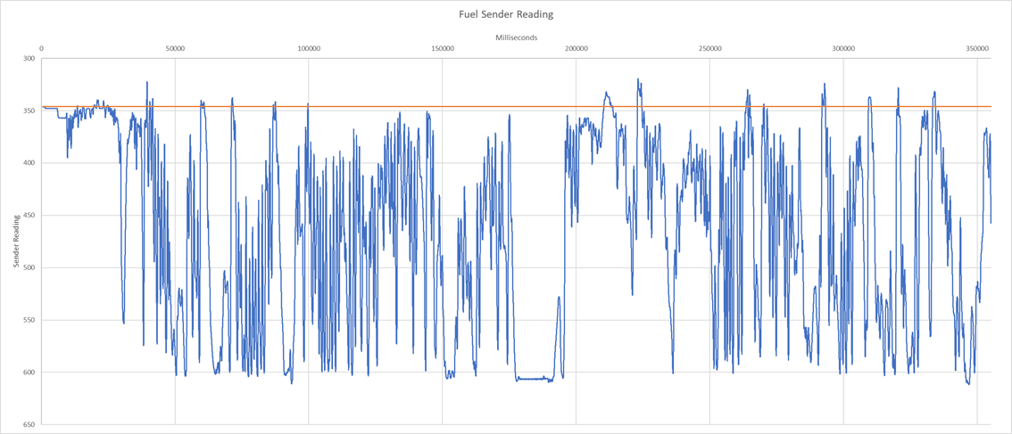
1. The signal was an awful lot messier than I had anticipated! As fuel slopped around in the tank the sender readings were swinging wildly all over the place. Hence the need for very heavy damping of the gauge response. The gauge was effectively extracting a long-term average out of that signal. I can see now that using a fairly coarse wire-wound resistor element in the sender isn’t a problem as it’s the average over a large range of values that gets reported in practice.
2. The orange line on the chart above shows the sender reading before I started driving, whilst the car was stationary and level in my garage. Note how the fuel level indicated by the sender almost never went above this whilst driving. Almost ALL of the readings were on the low side.
3. The low, flat bit in the centre of the chart corresponds to driving around a roundabout. This caused the fuel to be thrown to one side of the tank and the sender to bottom out.
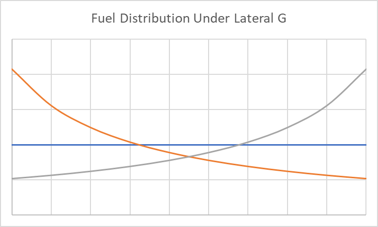
I think what is happening is something like what is shown in the chart below. This represents the fuel distribution laterally across the tank when stationary (blue line) or when turning left (grey line) or right (orange line). The area under each of these three lines is identical, representing the same total amount of fuel in the tank, but thrown to one side or the other when cornering. Note how a fuel tank sender near the centre line of the tank will always see a lower fuel level when the fuel is sloshing around than it will when stationary.
There’s not an awful lot I can do to compensate for this effect as pretty much ALL of the sender reading were skewed in the same direction and it’s pretty hard to work out the true fuel level from a set of readings which don’t even include that value in their range. I did look at just trying to work out whether the fuel level was steady or fluctuating, then adding a constant correction in the fluctuating case, but the effect does vary with the level of fuel in the tank and so it would need another calibration table, which would actually be very complicated to get data for, so I left that out for now at least. I did provide some rough compensation by allowing you to enter longer damping time constants for falling values than for rising values.